Image retrieval benchmark tutorial
- Retrieval benchmark
- Feature extractors algorithms comparison
- Average precisions
- Precision recall curves
- Retrieved images
- References
The source code of this tutorial is available in
retrievalDemo.m function, this text shows only
selected parts of the code.
The current implementation does not support Microsoft Windows platforms.
Retrieval benchmark
The image retrieval benchmark tests feature extractorss in a simple image retrieval system. The retrieval benchmark closely follows the work Jegou et. al [1]. First a set of local features is detected by selected feature extractor, and described using selected descriptor. To find most similar features it employs a K-Nearest neighbours search over descriptors from the all dataset images. Finally, a simple voting criterion based on K-nearest descriptors distances is used to sort the images (for the details c.f. [1]).
The dataset used in the evaluation consists of a set of images and a set of queries. Set of ground truth images for each query is split into three classes 'Good', 'Ok', 'Junk'. For each query, the average precision (area under the precision-recall curve) is calculated and averaged over all queries to get mean Average Precision (mAP) of the feature extractor.
Feature extractors algorithms comparison
The main purpose of this benchmark is to compare the feature extraction algorithms. In this tutorial we have selected feature extractors, which are part of the VLFeat library:
featExtractors{1} = VlFeatCovdet('method', 'hessianlaplace', ...
                                 'estimateaffineshape', true, ...
                                 'estimateorientation', false, ...
                                 'peakthreshold',0.0035,...
                                 'doubleImage', false);
featExtractors{2} = VlFeatCovdet('method', 'harrislaplace', ...
                                 'estimateaffineshape', true, ...
                                 'estimateorientation', false, ...
                                 'peakthreshold',0.0000004,...
                                 'doubleImage', false);
featExtractors{3} = VlFeatSift('PeakThresh',4);
The first two image feature extractors are affine covariant whereas the third one is just similarity invariant and is closely similar to Lowe's original SIFT feature extractor (DoG detector, in fact). All local features are described using by SIFT descriptor.
To perform the image retrieval benchmark we defined a subset of the original 'The Oxford Buildings' dataset to compute the results in a reasonable time.
dataset = VggRetrievalDataset('Category','oxbuild',...
                              'OkImagesNum',inf,...
                              'JunkImagesNum',100,...
                              'BadImagesNum',100);
The subset of Oxford buildings contains only 748 images as only a part of the 'Junk' and 'Bad' images is included. 'Bad' are images which does not contain anything from the queries. The original dataset consist of 5062 images.
Now an instance of a benchmark class is created. The benchmark computes
the nearest neighbours over all images. This can be too memory consuming,
however the search can be split into several parts and the results merged.
The parameter 'MaxNumImagesPerSearch' sets how many images are
processed at one KNN search.
retBenchmark = RetrievalBenchmark('MaxNumImagesPerSearch',100);
100 * 2000 * 128 * 4 ~ 100MB of memory
Given each image contains around 2000 features on average, each feature is
described by 128 bytes long descriptor and the fact that the used KNN
algorithm works only with single (4 Byte) values.
Finally we can run the benchmark:
for d=1:numel(featExtractors)
  [mAP(d) info(d)] =...
    retBenchmark.testFeatureExtractor(featExtractors{d}, dataset);
end
Even having a subset of the Oxford buildings dataset, it takes a while to evaluate the benchmark for selected feature extractors. The feature extraction for a single image takes several seconds so overall the feature extraction takes approximately:
3 � 748 � 3 = 6732s ~ 2h
Giving you a plenty of time for a coffee or even a lunch. Fortunately if
you have setup Matlab Parallel Computing Toolbox running this benchmark
with open matlabpool can run feature extraction and KNN
computation in parallel.
Both the features and partial KNN search results are stored in the cache so the computation can be interrupted and resumed at any time.
Average precisions
The results of the benchmark can be viewed at several levels of detail. The most general result is the mean Average Precision (mAP), a single value per a feature extractor. The mAPs can be visualises in a bar graph:
detNames = {'VLF-heslap', 'VLF-harlap', 'VLFeat-SIFT'};
bar(mAP);
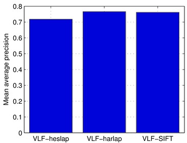
    VLF-heslap  VLF-harlap    VLF-SIFT
mAP      0.721       0.772       0.758
Note, that these values are computed only over small part of the Oxford Buildings dataset, and therefore are not directly comparable to the other state-of-the-art image retrieval systems run on the Oxford Buildings dataset. On the other hand this benchmark does not include any quantisation or spatial verification and thus is more focused on comparison of image features extractors.
An important measure in the features extractors comparison is a number of descriptors computed for each image, or average number of features per image. The average numbers of features can be easily obtained using:
numDescriptors = cat(1,info(:).numDescriptors);
numQueryDescriptors = cat(1,info(:).numQueryDescriptors);
avgDescsNum(1,:) = mean(numDescriptors,2);
avgDescsNum(2,:) = mean(numQueryDescriptors,2);
It can be seen that the selected set of feature extractors produce similar number of features with the selected settings:
                    VLF-heslap  VLF-harlap    VLF-SIFT
      Avg. #Descs.    1803.822    1678.195    1843.202
Avg. #Query Descs.     892.582     869.255     853.582
To get better insight where the extractors differ, we can plot the APs per
each query. These values are also contained in the info
structure. For example the APs for the first
15 queries can be visualised by:
queriesAp = cat(1,info(:).queriesAp); % Values from struct to single array
selectedQAps = queriesAp(:,1:15);     % Pick only first 15 queries
bar(selectedQAps');
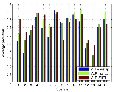
As you can see there are big differences between the queries. For example query number 8 as it is a query where the SIFT feature extractor gets much worse than other algorithms. Let's investigate the query number 8 in more detail. In the first step, we can show the precision recall curves.
Precision recall curves
The precision-recall curves are not part of the results but they can be
easily calculated using the RetrievalBenchmark.rankedListAp(query,
rankedList) static method.
queryNum = 8;
query = dataset.getQuery(queryNum);

for d=1:numel(featExtractors)
  % AP is calculated only based on the ranked list of retrieved images
  rankedList = rankedLists{d}(:,queryNum);
  [ap recall(:,d) precision(:,d)] = ...
    retBenchmark.rankedListAp(query, rankedList);
end

% Plot the curves
plot(recall, precision,'LineWidth',2);
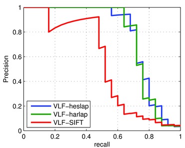
In this graph it can be seen that a VLF-SIFT (DoG + SIFT descriptor) achieved lower AP score because one of the first ranked images is wrong, therefore the area under the precision recall curve shrinks significantly.
We can check it by showing the retrieved images.
Retrieved images
The indices of the retrieved images are stored in
info.rankedList field. It contains indices of all dataset images
sorted by the voting score of each image. The details of the voting scheme can
be found in the help string of the retrieval benchmark class or in [1].
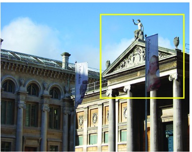
To asses the performance of the feature extractor, let's inspect the query number 8.
image(imread(dataset.getImagePath(query.imageId)));
% Convert query rectangle [xmin ymin xmax ymax] to [x y w h]
box = [query.box(1:2);query.box(3:4) - query.box(1:2)];
rectangle('Position',box,'LineWidth',2,'EdgeColor','y');
Having the ranked list we can show the retrieved images for all feature extractors.
rankedLists = {info(:).rankedList}; % Ranked list of the retrieved images
numViewedImages = 20;
for ri = 1:numViewedImages
  % The first image is the query image itself
  imgId = rankedList(ri+1);
  imgPath = dataset.getImagePath(imgId);
  subplot(5,numViewedImages/5,ri);
  subimage(imread(imgPath));
end
Images retrieved by the VLFeat Hessian Laplace:
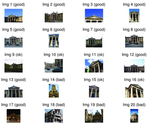
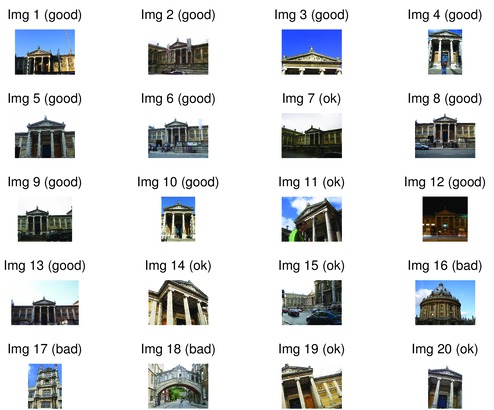
Image retrieved by the VLFeat Harris Laplace:
And finally, images retrieved by the VLFeat SIFT:
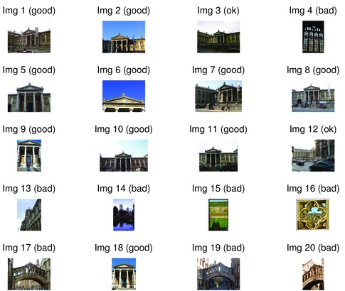
Observe that indeed the image ranked as the second is wrong for the VLF- SIFT feature extractor, consequently reducing its AP.
References
- H. Jegou, M. Douze, and C. Schmid. Exploiting descriptor distances for precise image search. Technical Report 7656, INRIA, 2011.