Table of Contents
The Local Invariant Order Pattern (LIOP) descriptor [32] is a local image descriptor based on the concept of local order pattern*. An order pattern is simply the order obtained by sorting selected image samples by increasing intensity. Consider in particular a pixel \(\bx\) and \(n\) neighbors \(\bx_1,\bx_2,\dots,\bx_n\). The local order pattern at \(\bx\) is the permutation \(\sigma\) that sorts the neighbours by increasing intensity \(I(\bx_{\sigma(1)}) \leq I(\bx_{\sigma(2)}) \leq \dots \leq I(\bx_{\sigma(2)})\).
An advantage of order patterns is that they are invariant to monotonic changes of the image intensity. However, an order pattern describes only a small portion of a patch and is not very distinctive. LIOP assembles local order patterns computed at all image locations to obtain a descriptor that at the same time distinctive and invariant to monotonic intensity changes as well as image rotations.
In order to make order patterns rotation invariant, the neighborhood of samples around \(\bx\) is taken in a rotation-covariant manner. In particular, the points \(\bx_1,\dots,\bx_n\) are sampled anticlockwise on a circle of radius \(r\) around \(\bx\), as shown in the following figure:
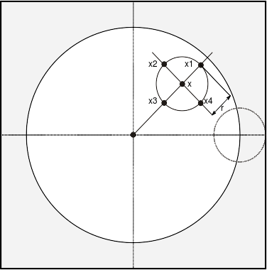
Since the sample points do not necessarily have integer coordinates, \(I(\bx_i)\) is computed using bilinear interpolation.
Intensity rank spatial binning
Once local order patterns are computed for all pixels \(\bx\) in the image, they can be pooled into a histogram to form an image descriptor. Pooling discards spatial information resulting in a warp-invariant statistics. In practice, there are two restriction on which pixels can be used for this purpose:
- A margin of \(r\) pixels from the image boundary must be maintained so that neighborhoods fall within the image boundaries.
- Rotation invariance requires the pooling regions to be rotation co-variant. A way to do so is to make the shape of the pooling region rotation invariant.
For this reason, the histogram pooling region is restricted to the circular region shown with a light color in the figure above.
In order to increase distinctiveness of the descriptor, LIOP pools multiple histograms from a number of regions \(R_1,\dots,R_m\) (spatial pooling). These regions are selected in an illumination-invariant and rotation-covariant manner by looking at level sets:
\[ R_t = \{\bx :\tau_{t} \leq I(\bx) < \tau_{t+1} \}. \]
In order to be invariant to monotonic changes of the intensity, the thresholds \(\tau_t\) are selected so that all regions contain the same number of pixels. This can be done efficiently by sorting pixels by increasing intensity and then partitioning the resulting list into \(m\) equal parts (when \(m\) does not divide the number of pixels exactly, the remaining pixels are incorporated into the last partition).
Weighted pooling
In order to compute a histogram of order pattern occurrences, one needs to map permutations to histogram bins. This is obtained by sorting permutation in lexycogrpahical order. For example, for \(n=4\) neighbors one has the following \(n!=24\) permutations:
| Permutation | Lexycographical rank |
|---|---|
| 1 2 3 4 | 1 |
| 1 2 4 3 | 2 |
| 1 3 2 4 | 3 |
| 1 3 4 2 | 4 |
| ... | ... |
| 4 3 1 2 | 23 |
| 4 3 2 1 | 24 |
In the following, \(q(\bx) \in [1, n!]\) will denote the index of the local order pattern \(\sigma\) centered at pixel \(\bx\).
The local order patterns \(q(\bx)\) in a region \(R_t\) are then pooled to form a histogram of size \(!n\). In this process, patterns are weighted based on their stability. The latter is assumed to be proportional to the number of pairs of pixels in the neighborhood that have a sufficiently large intensity difference:
\[ w(\bx) = \sum_{i=1}^n \sum_{j=1}^n [ |I(\bx_{i}) - I(\bx_{j})| > \Theta) ] \]
where \([\cdot]\) is the indicator function.
In VLFeat LIOP implementation, the threshold \(\Theta\) is either set as an absolute value, or as a faction of the difference between the maximum and minimum intensity in the image (restricted to the pixels in the light area in the figure above).
Overall, LIOP consists of \(m\) histograms of size \(n!\) obtained as
\[ h_{qt} = \sum_{\bx : q(\bx) = q \ \wedge\ \bx \in R_t} w(\bx). \]
Normalization
After computing the weighted counts \(h_{qt}\), the LIOP descriptor is obtained by stacking the values \(\{h_{qt}\}\) into a vector \(\mathbf{h}\) and then normalising it:
\[ \Phi = \frac{\mathbf{h}}{\|\mathbf{h}\|_2} \]
The dimensionality is therefore \(m n!\), where \(m\) is the numSpatialBins number of spatial bins and \(n\) is the numNeighbours number of neighbours (see vl_liopdesc_new). By default, this descriptor is stored in single format. It can be stored as a sequence of bytes by premultiplying the values by the constant 255 and then rounding:
\[ \operatorname{round}\left[ 255\, \times \Phi\right]. \]