This tutorial illustrates the use of the functions
vl_roc,
vl_det, and
vl_pr to generate ROC, DET, and precision-recall
curves.
VLFeat includes support for plotting starndard information retrieval curves such as the Receiver Operating Characteristic (ROC) and the Precision-Recall (PR) curves.
Consider a set of samples with labels labels and
score scores. scores is typically the output
of a classifier, with higher scores corresponding to positive
labels. Ideally, sorting the data by decreasing scores should leave
all the positive samples first and the negative samples last. In
practice, a classifier is not perfect and the ranking is not ideal.
The tools discussed in this tutorial allow to evaluate and visualize
the quality of the ranking.
For the sake of the illustration generate some data randomly as follows:
numPos = 20 ;
numNeg = 100 ;
labels = [ones(1, numPos) -ones(1,numNeg)] ;
scores = randn(size(labels)) + labels ;
In this case, there have five times more negative samples than positive ones. The scores are correlated to the labels as expected, but do not allow for a perfect separation of the two classes.
ROC and DET curves
To visualize the quality of the ranking, one can plot the ROC curve
by using the vl_roc
function:
vl_roc(labels, scores) ;
This produces the figure
The ROC curve is the parametric curve given by the true positve
rate (TPR) against the true negative rate (TNR). These two quantities
can be obtained from vl_roc as follows:
[tpr, tnr] = vl_roc(labels, scores) ;
The TPR value tpr(k) is the percentage of positive
samples that have rank smaller or equal than k (where
ranks are assigned by decreasing scores). tnr(k) is
instead the percentage of negative samples that have rank larger
than k. Therefore, if one classifies the samples with
rank smaller or equal than k to be positive and the rest
to be negative, tpr(k) and tnr(k) are
repsectively the probability that a positive/negative sample is
classified correctly.
Moving from rank k to rank k+1, if the
sample of rank k+1 is positive then tpr
increases; otherwise tnr decreases. An ideal classifier
has all the positive samples first, and the corresponding ROC curve is
one that describes two sides of the unit square.
The Area Under the Curve (AUC) is an indicator of the
overall quality of a ROC curve. For example, the ROC of the ideal
classifier has AUC equal to 1. Another indicator is the Equal
Error Rate (EER), the point on the ROC curve that corresponds to
have an equal probability of miss-classifying a positive or negative
sample. This point is obtained by intersecting the ROC curve with a
diagonal of the unit square. Both AUC and EER can be computed
by vl_roc:
[tpr, tnr, info] = vl_roc(labels, scores) ;
disp(info.auc) ;
disp(info.eer) ;
vl_roc has a couple of useful functionalities:
- Any sample with label equal to zero is effecitvely ignored in the evaluation.
- Samples with scores equal to
-inf are assumed to be never retrieved by the classifier. For these, the TNR is conventionally set to be equal to zero. - Additional negative and positive samples with
-inf score can be added to the evaluation by means of thenumNegatives andnumPositives options. For example,vl_roc(labels,scores,'numNegatives',1e4) sets the number of negative samples to 10,000. This can be useful when evaluating large retrieval systems, for which one may want to record inlabels andscores only the top ranked results from a classifier. - Different variants of the ROC plot can be produced. For example
vl_roc(labels,scores,'plot','tptn') swaps the two axis, plotting the TNR against the TPR. Since the TPR is also the recall (i.e., the percentage of positive samples retrieved up to a certain rank), this makes the plot more directly comparable to a precision-recall plot.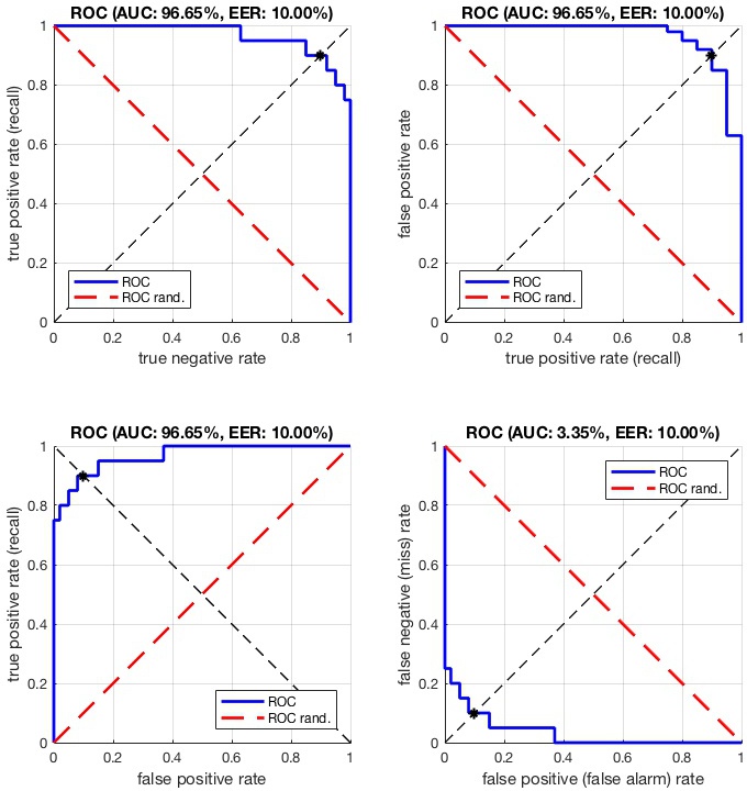 Variants of the ROC plot.
A limitation of the ROC curves in evaluating a typical retrieval system is that they put equal emphasis on false positive and false negative errors. In a tipical retrieval application, however, the vast majority of the samples are negative, so the false negative rate is typically very small for any operating point of interest. Therefore the emphasis is usually on the very first portion of the rank, where the few positive samples should concentrate. This can be emphasized by using either precision-recall plot or a variant of the ROC curves called Detection Error Tradeoff (DET) curves.
A DET curve plots the FNR (also called false alarm rate)
against teh FPR (also called miss rate) in logarithmic
coordiantes. It can be generated
by vl_det function
call:
Precision-recall curves
Both ROC and DET curves normalize out the relative proportions of
positive and negative samples. By contrast, a Precision-Recall
(PR) curve reflects this directly. One can plot the PR curve by
using the vl_pr
function:
vl_pr(labels, scores) ;
This produces the figure
The PR curve is the parametric curve given by precision and
recall. These two quantities can be obtained from vl_roc
as follows:
[recall, precision] = vl_roc(labels, scores) ;
The precision value precision(k) is the proportion of
samples with rank smaller or equal than k-1 that are
positive(where ranks are assigned by decreasing
scores). recall(k) is instead the percentage of positive
samples that have rank smaller or equal than k-1. For
example, if the first two samples are one positive and one
negative, precision(3) is 1/2. If there are in total 5
positive samples, then recall(3) is 1/5.
Moving from rank k to rank k+1, if the
sample of rank k+1 is positive then
both precision and recall increase;
otherwise precision decreases and recall
stays constant. This gives the PR curve a characteristic
saw-shape. For aan ideal classifier that ranks all the positive
samples first the PR curve is one that describes two sides of the unit
square.
Similar to the ROC curves, the Area Under the Curve (AUC)
can be used to summarize the quality of a ranking in term of precision
and recall. This can be obtained as info.auc by
[rc, pr, info] = vl_pr(labels, scores) ;
disp(info.auc) ;
disp(info.ap) ;
disp(info.ap_interp_11) ;
The AUC is obtained by trapezoidal interpolation of the precision.
An alternative and usually almost equivalent metric is the Average
Precision (AP), returned as info.ap. This is the
average of the precision obtained every time a new positive sample is
recalled. It is the same as the AUC if precision is interpolated by
constant segments and is the definition used by TREC most
often. Finally, the 11 points interpolated average precision,
returned as info.ap_interp_11. This is an older TREC
definition and is obtained by taking the average of eleven precision
values, obtained as the maximum precision for recalls largerer than
0.0, 0.1, ..., 1.0. This particular metric was used, for example, in
the PASCAL VOC challenge until the 2008 edition.