Table of Contents
This tutorial introduces the vl_covdet VLFeat command
implementing a number of co-variant feature detectors and
corresponding descriptors. This family of detectors
include SIFT as well as multi-scale conern
(Harris-Laplace), and blob (Hessian-Laplace and Hessian-Hessian)
detectors. For example applications, see also
the SIFT tutorial.
Extracting frames and descriptors
The first example shows how to
use vl_covdet to compute
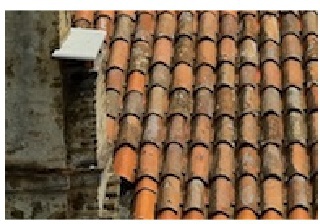
and visualize co-variant features. Fist, let us load an example image
and visualize it:
im = vl_impattern('roofs1') ;
figure(1) ; clf ;
image(im) ; axis image off ;
The image must be converted to gray=scale and single precision. Then
vl_covdet can be called in order to extract features (by
default this uses the DoG cornerness measure, similarly to SIFT).
imgs = im2single(rgb2gray(im)) ;
frames = vl_covdet(imgs, 'verbose') ;
The verbose option is not necessary, but it produces
some useful information:
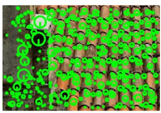
vl_covdet: doubling image: yes
vl_covdet: detector: DoG
vl_covdet: peak threshold: 0.01, edge threshold: 10
vl_covdet: detected 3518 features
vl_covdet: kept 3413 inside the boundary margin (2)
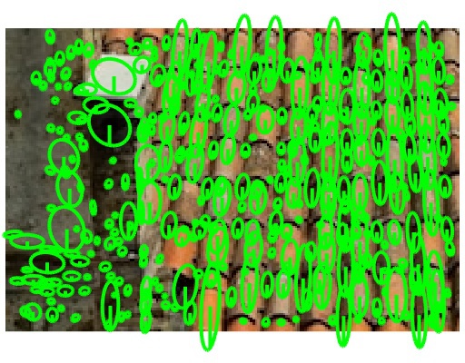
The vl_plotframe command can then be used to plot
these features
hold on ;
vl_plotframe(frames) ;
which results in the image
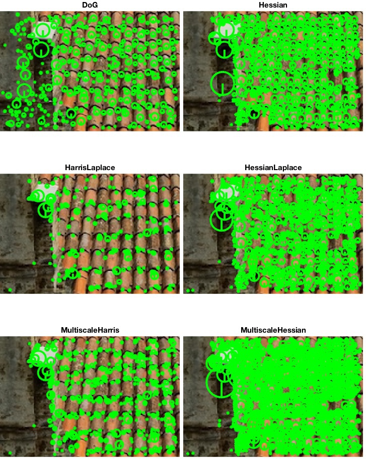
In addition to the DoG detector, vl_covdet supports a
number of other ones:
- The Difference of Gaussian operator (also known as trace of the Hessian operator or Laplacian operator) uses the local extrema trace of the multiscale Laplacian operator to detect features in scale and space (as in SIFT).
- The Hessian operator uses the local extrema of the mutli-scale determinant of Hessian operator.
- The Hessian Laplace detector uses the extrema of the multiscale determinant of Hessian operator for localisation in space, and the extrema of the multiscale Laplacian operator for localisation in scale.
- Harris Laplace uses the multiscale Harris cornerness measure instead of the determinant of the Hessian for localization in space, and is otherwise identical to the previous detector..
- Hessian Multiscale detects features spatially at multiple scales by using the multiscale determinant of Hessian operator, but does not attempt to estimate their scale.
- Harris Multiscale is like the previous one, but uses the multiscale Harris measure instead.
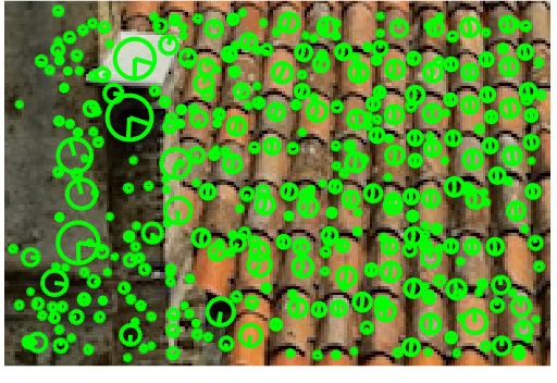
For example, to use the Hessian-Laplace operator instead of DoG, use the code:
frames = vl_covdet(imgs, 'method', 'HarrisLaplace') ;
The following figure shows example of the output of these detectors:
Understanding feature frames
To understand the rest of the tutorial, it is important to
understand the geometric meaning of a feature frame. Features
computed by vl_covdet are oriented ellipses and
are defined by a translation $T$ and linear map $A$ (a $2\times 2$)
which can be extracted as follows:
 T = frame(1:2) ;
 A = reshape(frame(3:6),2,2)) ;
The map $(A,T)$ moves pixels from the feature frame (also called normalised patch domain) to the image frame. The feature is represented as a circle of unit radius centered at the origin in the feature reference frame, and this is transformed into an image ellipse by $(A,T)$.
In term of extent, the normalised patch domain is a square box centered at the origin, whereas the image domain uses the standard MATLAB convention and starts at (1,1). The Y axis points downward and the X axis to the right. These notions are important in the computation of normalised patches and descriptors (see later).
Affine adaptation
Affine adaptation is the process of estimating the affine shape of an image region in order to construct an affinely co-variant feature frame. This is useful in order to compensate for deformations of the image like slant, arising for example for small perspective distortion.
To switch on affine adaptation, use
the EstimateAffineShape option:
frames = vl_covdet(imgs, 'EstimateAffineShape', true) ;
which detects the following features:
Feature orientation
The detection methods discussed so far are rotationally invariant. This means that they detect the same circular or elliptical regions regardless of an image rotation, but they do not allow to fix and normalise rotation in the feature frame. Instead, features are estimated to be upright by default (formally, this means that the affine transformation $(A,T)$ maps the vertical axis $(0,1)$ to itself).
Estimating and removing the effect of rotation from a feature frame
is needed in order to compute rotationally invariant descriptors. This
can be obtained by specifying the EstimateOrientation
option:
frames = vl_covdet(imgs, 'EstimateOrientation', true, 'verbose') ;
which results in the following features being detected:
The method used is the same as the one proposed by D. Lowe: the orientation is given by the dominant gradient direction. Intuitively, this means that, in the normalized frame, brighter stuff should appear on the right, or that there should be a left-to-right dark-to-bright pattern.
In practice, this method may result in an ambiguous detection of the orientations; in this case, up to four different orientations may be assigned to the same frame, resulting in a multiplication of them.
Computing descriptors
vl_covdet can also compute descriptors. Three are
supported so far: SIFT, LIOP and raw patches (from which any other
descriptor can be computed). To use this functionality simply add an
output argument:
[frames, descrs] = vl_covdet(imgs) ;
This will compute SIFT descriptors for all the features. Each
column of descrs is a 128-dimensional descriptor vector
in single precision. Alternatively, to compute patches use:
[frames, descrs] = vl_covdet(imgs, 'descriptor', 'liop') ;
Using default settings, each column will be a 144-dimensional descriptor vector in single precision. If you wish to change the settings, use arguments described in LIOP tutorial
[frames, descrs] = vl_covdet(imgs, 'descriptor', 'patch') ;
In this case each column of descrs is a stacked patch.
To visualize the first 100 patches, one can use for example:
w = sqrt(size(patches,1)) ;
vl_imarraysc(reshape(patches(:,1:10*10), w,w,[])) ;


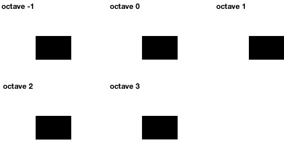
There are several parameters affecting the patches associated to
features. First, PatchRelativeExtent can be used to
control how large a patch is relative to the feature scale. The extent
is half of the side of the patch domain, a square in
the frame reference
frame. Since most detectors latch on image structures (e.g. blobs)
that, in the normalised frame reference, have a size comparable to a
circle of radius one, setting PatchRelativeExtent to 6
makes the patch about six times largerer than the size of the corner
structure. This is approximately the default extent of SIFT feature
descriptors.
A second important parameter is PatchRelativeSigma
which expresses the amount of smoothing applied to the image in the
normalised patch frame. By default this is set to 1.0, but can be
reduced to get sharper patches. Of course, the amount of
smoothing is bounded below by the resolution of the input image: a
smoothing of, say, less than half a pixel cannot be recovered due to
the limited sampling rate of the latter. Moreover, the patch must be
sampled finely enough to avoid aliasing (see next).
The last parameter is PatchResolution. If this is
equal to $w$, then the patch has a side of $2w+1$ pixels. (hence the
sampling step in the normalised frame is given by
PatchRelativeExtent/PatchResolution).
Extracting higher resolution patches may be needed for larger extent
and smaller smoothing. A good setting for this parameter may be
PatchRelativeExtent/PatchRelativeSigma.
Custom frames
Finally, it is possible to use vl_covdet to compute
descriptors on custom feature frames, or to apply affine adaptation
and/or orientation estimation to these.
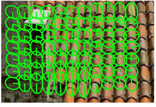
For example
delta = 30 ;
xr = delta:delta:size(im,2)-delta+1 ;
yr = delta:delta:size(im,1)-delta+1 ;
[x,y] = meshgrid(xr,yr) ;
frames = [x(:)'; y(:)'] ;
frames(end+1,:) = delta/2 ;

[frames, patches] = vl_covdet(imgs, ...
                              'frames', frames, ...
                              'estimateAffineShape', true, ...
                              'estimateOrientation', true) ;
computes affinely adapted and oriented features on a grid:
Getting the scale spaces
vl_covdet can return additional information about the
features, including the scale spaces and scores for each detected
feature. To do so use the syntax:
[frames, descrs, info] = vl_covdet(imgs) ;
This will return a structure info
info =

                    gss: [1x1 struct]
                    css: [1x1 struct]
             peakScores: [1x351 single]
             edgeScores: [1x351 single]
       orientationScore: [1x351 single]
    laplacianScaleScore: [1x351 single]
The last four fields are the peak, edge, orientation, and Laplacian scale scores of the detected features. The first two were discussed before, and the last two are the scores associated to a specific orientation during orientation assignment and to a specific scale during Laplacian scale estimation.
The first two fields are the Gaussian scale space and the
cornerness measure scale space, which can be plotted by means
of vl_plotss. The following is the of the Gaussian scale
space for our example image:
The following is an example of the corresponding cornerness measure: